
(1)
Reaction-Diffusion Texture Generation on GPU
Introduction
Nowadays, computers are used all around us, at work, when we are on the road, but increasingly often in our houses as well. Gaming on either a personal computer or gaming console is enjoying its finest hour as one or more gaming platforms can be found in many homes. To keep up with the demand for better games that contain realistic graphics technology improves at a constant pace. These improvements have led to the introduction of a technique called shaders.
Shaders are small programs that execute on the graphics processing unit (GPU) at different places of the rendering pipeline. Their intended purpose was for game developers to take some load from the CPU to the GPU, especially in regard to intense graphics operations. This has caused the quality and realism of the graphics to improve tremendously. It was quickly discovered that shaders could also be used for general purpose calculations (GPGPU). Because computations on the GPU take the load of calculations on the CPU, it is interesting to show how an often recurring problem, i.e.: solving partial differential equations, can be solved on the GPU. This is the focus of the application of shaders in this article.
Texture differentiation between objects in a scene can, in some circumstances, increase realism. For example, imagine a scene in which a harem of zebras crosses a beautiful plain. As you might know, each zebra has its own distinct black and white striped pattern, so each animal in our scene should have a unique striped pattern. To have an artist create all these different textures could be very time consuming.
This article focuses on procedural texture generation using a reaction-diffusion (RD) system [1]. This system is able to generate textures based on a number of parameters provided by the user. RD could be used to generate the stripes on each zebra automatically. Source code for a conventional implementation for the CPU as well as an implementation for the GPU is provided. The techniques described in this article can easily be applied to any other discretizable two-dimensional partial differential equation one would like to solve (such as the wave equation).
Reaction-diffusion
A reaction-diffusion model is a mathematical representation of a natural phenomenon. It is described by a reaction that occurs between at least two fluids at differing concentrations, diffusing and dissipating through time by iterating over a discritized sample area.
This section introduces this model in detail. Without meddling with the formulas too much, the model is discretized into an iterative process which eventually will be implemented in a GPU fragment shader.
The simplest form of the reaction-diffusion equation is shown in (1) and (2):
(1)
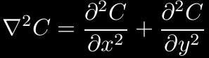
(2)
C' is the time derivative of C, a field or function that contains the concentrations of a certain fluid. This fluid develops over time using three different parameters: a is the amount with which the fluid will diffuse over time, b represents the ratio of dissipation and finally R represents the concentration added at every position depending on the restrictions set by the function.
To be able to approximate the solution of the partial differential equation written in full in (2) we introduce a NxN discretization of the field that contains the concentrations for a finite number of points. This discretization can be viewed as a mesh of points that overlays the actual field. Each point is influenced by their neighbours. As (3) shows, the Laplacian of C i, j is calculated by taking the values of surrounding points and dividing them by the square of the step in space that is taken between each discretized point h.
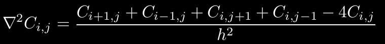
(3)
This formula can also be written or as a convolution matrix. Combining them with variables a and b the convolution matrix M is formed.
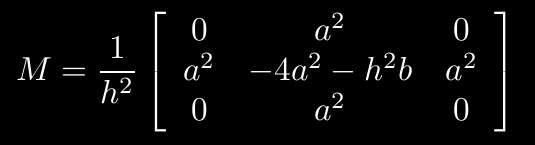
(4)
The paper from which this model is taken contains a number of extensions to this very basic model allowing for diffusion limitations at certain angles and introducing diffusion mappings to create space-varying diffusions. However, for simplicity's sake we will just stick to this isotropic model.
Now, we've got a convolution matrix M, using Euler integration we can calculate C t+1 from C t as follows:

(5)
The one thing we have yet to talk about is the reaction function R. This function returns a number dependent on the values in the reaction-diffusion system at a specific field position (x, y), at some point in time (t); the function takes three parameters: R(x, y, t).
The reaction in our implementation will be very simple. There shall be two different fields with fluids, C + and C -. If the concentration of C + at position (x, y) is bigger than that of C - at the same position, then the constant k will be added at that location. This is the reaction function for C + and C -.
function R(x, y, t) : int
begin
  if C+(x, y) > C-(x, y):
    return k;
  return 0;
end
Okay, take a deep breath. This was all the math you will see in this article. I realize there were no explanations, but this article focusses on simple GPGPU operations. If you want to know more, I suggest you read the paper referenced by this article. To discover how one could implement this in a very straight-forward/unoptimized way on a CPU, check out the source that is included with this article.
GPU Technique
As described in the introduction of this article, the simple isotropic reaction-diffusion system will be implemented in a fragment shader that is executed on the GPU. To achieve this goal the coming section will explain the techniques that are used in the GPU implementation.
For completeness' sake, this section starts with a short introducation to shaders. Secondly the ping-pong technique is explained. Thirdly, framebuffer objects (FBO) are explained as they are necessary to implement ping-ponging on a GPU. The tools used in this article are OpenGL in combination with NVIDIA's Cg shader language, and C++ to combine it all into a neat little packet of working code.
Shaders
There are two types of shaders: vertex- and fragment shaders. They are located at different places in the rendering pipeline. Vertex shaders are able to influence the properties of vertices that are passed by the developer through the pipeline. Things such as vertex position and color can be changed depending on the functionality of the vertex shader. A fragment shader is invoked for every pixel that is drawn to the framebuffer, they influence the color that will be drawn onto the current buffer. In this article, the pixel values the fragment shader writes to the framebuffer are the result of a calculation in our reaction-diffusion system.
Ping-Pong
As you might have noticed from the discretized version of the reaction-diffusion system, the system's results are achieved by iterating over the field a number of times. Advancing the fluid concentrations over time means that C t+1 is calculated using C t. To calculate the step after that, C t + 1 becomes C t, and the process is repeated until the desired result is achieved. In our CPU implementation we use two NxN fields of doubles to achieve this type of iteration. Once the calculations of one iteration have completed, the pointers to the fields are flipped so the C t+1 now represents C t.
Framebuffer Objects
The obvious choice for a field of values on a graphics card is a texture of N by N pixels. The NVIDIA card used during the implementation of this application (a 6600GT) supports a type of texture that only has one color channel (red), and uses a high-precision floating point format for its contents. The precision offered by this format is enough for our purposes [1].
Testing the more complicated anisotropic variant of the RD model led me to believe that a more precise texture format would be necessary to successfully implement it.
Putting information into textures is usually performed at initialization using the glTexImage2D function. Unfortunately this is not an option for us, as such operations are slow, thereby defeating the purpose of implementing reaction-diffusion on the GPU.
A fragment shader outputs pixel colors to the screen. Wouldn't it be great if that information could directly be stored in a texture? This way it could be used during later GPU operations without having to transfer any information from and to the CPU, greatly increasing the performance of the application. Fortunately for us, this is possible by using framebuffer objects (FBOs) [2]. The implementation offers a simple reusable implementation of an OpenGL FBO.
A framebuffer object is an extension to the OpenGL library. One can look at it as a container for different elements of an OpenGL context. When a framebuffer object is created, no elements are attached. Textures can be attached to these framebuffers as color attachments, which are areas on which the framebuffer will write output. This mechanism allows us to directly render geometry to a texture. To create a texture filled with calculations of the RD system, one quad of N by N pixels is drawn onto a framebuffer with a color attachment. For each point in this quad the fragment shader will calculate the value of the next timestep. After the quad has been drawn completely, all values for the next timestep are known and stored inside our texture.
It is possible to attach more than one color attachment to a framebuffer object. To select the active color attachment, the one that is drawn to, the glDrawBuffer function is used. It is used to our advantage in the implementation of the reaction-diffusion system for the GPU by performing ping-pong on the texture IDs acquired when creating the textures.
Implementation
To give you an idea of how the implementation of this technique works, this section will provide a short tour through the source code of the GPU implementation of the reaction-diffusion algorithm and finally provide you with a number of screenshots.
There are two different fragment shaders that are used in the implementation. The first shader contains code that will change the values in the color attachments to the next time step. Visualization of the values within the fluids of the RD system is provided by the second fragment shader. The shaders can be found in the cg/ directory.
The main-loop (found in main.cpp) performs one iteration for both fluids (C - and C +) after which the buffers are rotated. The step method in the RDsystem class associates the textures of both concentrations with a uniform parameter in the fragment shader that solves the equations.
g_plus->step(g_min->current(), g_plus->current());
g_min->step(g_min->current(), g_plus->current());
g_min->rotate();
g_plus->rotate();
Figure 1 shows the steps necessary to succesfully calculate the values of the next timestep using a fragment shader. First, the fragment shader is activated; then the variables that are associated with and used inside the fragment shader are set-up.
Take extra care when you setup a texture parameter using the Cg toolkit. These parameters need to be explicitely enabled and disabled, before and after using them.
The next step is to change the framebuffer object onto which the quad will be drawn; after which the proper color attachment is selected. When we've reached this point without errors, everything has been set-up properly. We can now render a quad to the framebuffer. Each point that is rendered represents one element of the next timestep.
After the quad was drawn the elements that were intialized, are uncoupled and destroyed in reversed order.
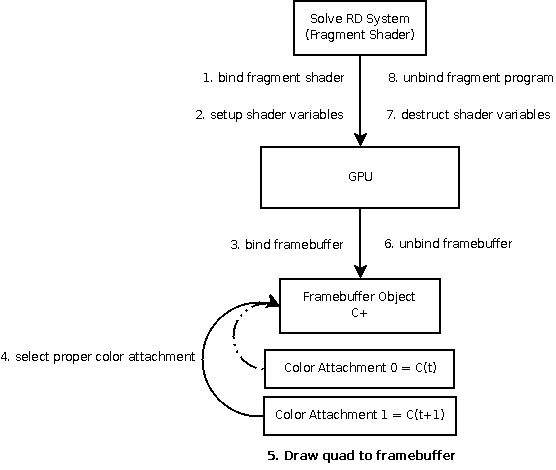
Figure 1: Sequence of actions necessary to calculate the next timestep of an RD field.
Results
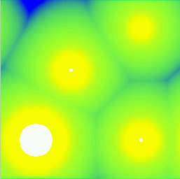
This paragraph is where I get to show some of the results that have been achieved by using CPU and GPU-based approaches of a reaction-diffusion system. The picture at the top left shows the output of our first, CPU-based, implementation of the isotropic RD algorithm.
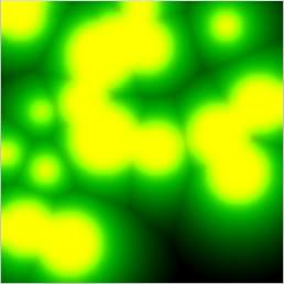
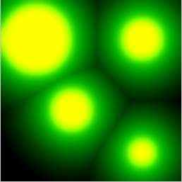
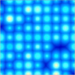
The remaining screenshots are outputs from the fragment shader implementation. As you can see, the pictures resemble cell structures, this becomes most apparent in the last two pictures. When the concentrations fields dissipate over time, and encounter other concentrations, they will stop to leak into the environment in that direction, thereby forming a kind of barrier that resembles the border of a cell.
As this implementation only shows the isotropic implementation of the RD system the results are quite basic. However, when one implements more advanced features such as dissipation direction limitations, found in the anisotropic variant, much more varied results can be achieved.
Conclusion
As the hardware on our graphic cards becomes more powerful, moving certain calculations to the GPU makes a lot of sense. As this article has shown, one can easily implement discretizations of partial differential equations on the GPU. They are encountered in many areas of computer science.
The technique used to achieve a result over time through iteration uses a framebuffer and two color attachments in the form of floating point textures. Each texture is a representation of a state of the system, either at time t or t + 1. Ping-ponging textures allows the discretized field to progress in time.
Especially on newer graphics hardware the implementation attached to this article is considerably faster than the conventional implementation. Keep in mind though, that no mathematical optimizations were performed to enhance its behaviour. Such optimizations could probably considerably performance of both approaches.
Even though we didn't manage to bring the stripes of our zebras from the introduction on the screen, the screenshots show that even a simple model can create visually pleasing results. To actually create the zebra textures, one would have to implement the extensions offered by [1].
By manipulating:
- the places at which the fluids are initialized;
- how much of the fluids is available;
- the amount of iterations that are allowed to occur;
- and the fluids visualisation.
Even a simple isotropic reaction-diffusion model such as the one described in this article is able to generate pretty results in a timely manner.
Questions and/or mistakes in this article can be reported to marnixkok@gmail.com.
References
[1] Reaction-Diffusion Textures written by Andrew Witkin and Michael Kass published in Computer Graphics #25. http://www.cs.cmu.edu/afs/cs/user/aw/www/pdf/texture.pdf
[2] The OpenGL Framebuffer Object Extension; by Simon Green, NVIDIA Corporation http://http.download.nvidia.com/developer/presentations/2005/GDC/OpenGL_Day/OpenGL_FrameBuffer_Object.pdf